Scrapy + Python 3: PTT Data Scraping and Analysis

Scrapy 1.1 with Python 3 Support

Long long time ago, I wanted to learn about web crawling to scrape some data from the PTT forum to see what could be done with it. I found the Scrapy framework, and felt it had great potential. But it didn’t support Python 3 at that time, so I’ve decided to wait.

Now, Scrapy 1.1 is released. Along with updated features, it also has basic Python 3 support. So I’ve decided to test about it and start writing a web scraper.

Environment Setup

Because I am going to scrape data from PTT forum, I’ve decided to build my service on the machine inside NTU CS to minimize the possibility to be banned. I also set up a higher delay to prevent too many multiple concurrent connections.

If you are using your own machine, you might need to install some additional packages:

sudo apt-get install python3-dev libxml2-dev libxslt1-dev zlib1g-dev libffi-dev libssl-dev

Now, we create our virtual environment using pyvenv so as to install our own packages:

pyvenv-3.5 my_env
source my_env/bin/activate

pip install -U pip

Afterwards, install all the packages that are needed:

# For some reasons, I need to use `python /sbin/pip3.5` instead of the following command on the machine
pip install Scrapy==1.1.0 numpy notebook scipy scikit-learn seaborn jieba

Building the Scraper

After reading the tutorial, I would start building my first Scrapy crawler!

Firstly, create a project:

scrapy startproject ptt

Set up download delay:

# <root_dir>/ptt/settings.py
DOWNLOAD_DELAY = 1.25

Define some fields to extract, including content and comments:

# <root_dir>/ptt/items.py
class PostItem(scrapy.Item):
    title = scrapy.Field()
    author = scrapy.Field()
    date = scrapy.Field()
    content = scrapy.Field()
    comments = scrapy.Field()
    score = scrapy.Field()
    url = scrapy.Field()

Start modifying <root_dir>/ptt/spiders/ptt.py to actually build the scraper.

Firstly, let’s test if we could actually connect to PTT:

import scrapy

class PTTSpider(scrapy.Spider):
    name = 'ptt'
    allowed_domains = ['ptt.cc']
    start_urls = ('https://www.ptt.cc/bbs/Gossiping/index.html', )

    def parse(self, response):
        filename = response.url.split('/')[-2] + '.html'
        with open(filename, 'wb') as f:
            f.write(response.body)

On the <root_dir> directory (which contains scrapy.cfg), execute the following to start the program:

scrapy crawl ptt

After it finished, we should find a HTML file on the current directory. The page asks us whether we are older than 18 years old. In order to successfully scrape articles from the Gossiping board on PTT, we need to automatically answer this form in our program. Although we could also use cookies to pretend we have answered it, here I will actually submit the form to mimic human behaviour. (Scrapy would save the cookies generated during the process between connections.)

Automatically Answer the Age Question

So we add a test to detect whether we are in the age question page by the div.over18-notice element. Here we use XPath to specify the exact position of the element. I first knew about XPath while I was doing intern at Microsoft, so it feels familiar.

import logging

from scrapy.http import FormRequest

class PTTSpider(scrapy.Spider):
    # ...
    _retries = 0
    MAX_RETRY = 1

    def parse(self, response):
        if len(response.xpath('//div[@class="over18-notice"]')) > 0:
            if self._retries < PTTSpider.MAX_RETRY:
                self._retries += 1
                logging.warning('retry {} times...'.format(self._retries))
                yield FormRequest.from_response(response,
                                                formdata={'yes': 'yes'},
                                                callback=self.parse)
            else:
                logging.warning('you cannot pass')

        else:
          # ...

We utilize FormRequest to send the form, and use callback to get back to parse after form is submitted. In case the attempt failed and we locked ourself into repeat submission of the form, I also use MAX_RETRY to restrict the number of submissions.

Automatically Crawl Every Article and Go to Next Pages

Next, let’s build a spider to extract links for the posts. Here we also use CSS Selector, css('.r-ent > div.title > a::attr(href)') to get the links of the articles. Afterwards, we use response.urljoin to convert relative URLs to absolute URLs and pass them to parse_post for further processing.

class PTTSpider(scrapy.Spider):
    # ...

    _pages = 0
    MAX_PAGES = 2

    def parse(self, response):
        if len(response.xpath('//div[@class="over18-notice"]')) > 0:
            # ...
        else:
            self._pages += 1
            for href in response.css('.r-ent > div.title > a::attr(href)'):
                url = response.urljoin(href.extract())
                yield scrapy.Request(url, callback=self.parse_post)

            if self._pages < PTTSpider.MAX_PAGES:
                next_page = response.xpath(
                    '//div[@id="action-bar-container"]//a[contains(text(), "上頁")]/@href')
                if next_page:
                    url = response.urljoin(next_page[0].extract())
                    logging.warning('follow {}'.format(url))
                    yield scrapy.Request(url, self.parse)
                else:
                    logging.warning('no next page')
            else:
                logging.warning('max pages reached')

Finally, we use XPath to extract the link to next page, and automatically follow the pages. MAX_PAGES is used to control the maximum number of pages to follow.

Actually Scrape the Posts

Finally, let’s actually download the posts. We would extract title, author, content, and comments. In addition, we record the positivity and negativity for each comment as well as for the post.

import datetime

from ptt.items import PostItem

class PTTSpider(scrapy.Spider):
    # ...
    def parse_post(self, response):
        item = PostItem()
        item['title'] = response.xpath(
            '//meta[@property="og:title"]/@content')[0].extract()
        item['author'] = response.xpath(
            '//div[@class="article-metaline"]/span[text()="作者"]/following-sibling::span[1]/text()')[
                0].extract().split(' ')[0]
        datetime_str = response.xpath(
            '//div[@class="article-metaline"]/span[text()="時間"]/following-sibling::span[1]/text()')[
                0].extract()
        item['date'] = datetime.strptime(datetime_str, '%a %b %d %H:%M:%S %Y')

        item['content'] = response.xpath('//div[@id="main-content"]/text()')[
            0].extract()

        comments = []
        total_score = 0
        for comment in response.xpath('//div[@class="push"]'):
            push_tag = comment.css('span.push-tag::text')[0].extract()
            push_user = comment.css('span.push-userid::text')[0].extract()
            push_content = comment.css('span.push-content::text')[0].extract()

            if '推' in push_tag:
                score = 1
            elif '噓' in push_tag:
                score = -1
            else:
                score = 0

            total_score += score

            comments.append({'user': push_user,
                             'content': push_content,
                             'score': score})

        item['comments'] = comments
        item['score'] = total_score
        item['url'] = response.url

        yield item

Finally, execute the following command. The crawler would start to scrape the posts and save them into a big JSON file:

scrapy crawl ptt -o gossip.json

Data Analysis in IPython Notebook

After we downloaded the posts, we could start data analysis. In this experiment, I downloaded 1881 articles from the Gossiping board on PTT. We will use IPython Notebook to do data analysis, the experiment could be viewed on PTT Analysis @ nbviewer.

Because I found the figures built with Seaborn seems to be more pretty when I was watching CS 109 videos, I would try it in this experiment as well.

We will use the following packages:

Firstly load all packages:

%matplotlib notebook

import json

from collections import defaultdict

import jieba
import matplotlib.pyplot as plt
import numpy as np
import seaborn as sns

from sklearn.feature_extraction import DictVectorizer
from sklearn.feature_extraction.text import TfidfTransformer
from sklearn.svm import LinearSVC

sns.set(style='whitegrid')

And then load the articles:

# load ptt posts

path = 'gossip.json'

with open(path) as f:
    posts = json.load(f)

Comments Analysis

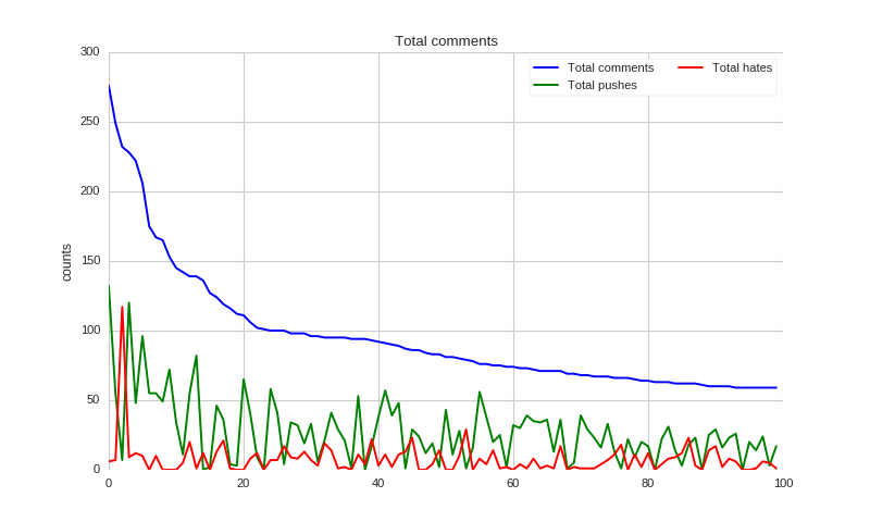
Let’s first figure out how many comments everyone has. Maybe this shows how addicted everyone is to PTT. But due to privacy concern, I would not display the actual IDs here. Firstly, compute the number of comments:

# get pushes

total_comments = defaultdict(int)
total_pushes = defaultdict(int)
total_hates = defaultdict(int)

for post in posts:
    for comment in post['comments']:
        user = comment['user']
        total_comments[user] += 1

        if comment['score'] > 0:
            total_pushes[user] += 1

        elif comment['score'] < 0:
            total_hates[user] += 1

And then we could draw a figure the show the most active users.

def show_distributions(counts, pushes, hates):
    sorted_cnts = [t[0] for t in sorted(counts.items(), key=lambda x: -x[1])][:100]
    y = [counts[u] for u in sorted_cnts]
    y_pushes = [pushes[u] for u in sorted_cnts]
    y_hates = [hates[u] for u in sorted_cnts]
    x = range(len(y))

    f, ax = plt.subplots(figsize=(10, 6))

    sns.set_color_codes('pastel')
    sns.plt.plot(x, y, label='Total {}'.format('comments'), color='blue')
    sns.plt.plot(x, y_pushes, label='Total {}'.format('pushes'), color='green')
    sns.plt.plot(x, y_hates, label='Total {}'.format('hates'), color='red')

    ax.legend(ncol=2, loc='upper right', frameon=True)
    ax.set(ylabel='counts',
           xlabel='',
           title='Total comments')
    sns.despine(left=True, bottom=True)

    plt.show(f)

# display pushes
show_distributions(total_comments, total_pushes, total_hates)

As we could see, most users have positive comments, but there are also some users post a lot of negative comments!

How Many Users Have a Specific Number of Comments?

Word Analysis

Let’s see what kinds of words are strongly correlated to negative and positive responses. And what kinds of words are most frequently used in positive and negative comments.

Firstly, use Jieba segmenter to segment the texts and collect the words. We also record the positivity and negativity of each article.

# grap post
words = []
scores = []

for post in posts:
    d = defaultdict(int)
    content = post['content']
    if post['score'] != 0:
        for l in content.split('\n'):
            if l:
                for w in jieba.cut(l):
                    d[w] += 1
        if len(d) > 0:
            words.append(d)
            scores.append(1 if post['score'] > 0 else 0)

We also process comments in the same way.

# grap comments
c_words = []
c_scores = []

for post in posts:
    for comment in post['comments']:
        l = comment['content'].strip()
        if l and comment['score'] != 0:
            d = defaultdict(int)
            for w in jieba.cut(l):
                d[w] += 1
            if len(d) > 0:
                c_scores.append(1 if comment['score'] > 0 else 0)
                c_words.append(d)

Finally, use TfidfTransformer to build the feature vector, and use LinearSVC to train a classifier,

# convert to vectors
dvec = DictVectorizer()
tfidf = TfidfTransformer()
X = tfidf.fit_transform(dvec.fit_transform(words))

c_dvec = DictVectorizer()
c_tfidf = TfidfTransformer()
c_X = c_tfidf.fit_transform(c_dvec.fit_transform(c_words))

svc = LinearSVC()
svc.fit(X, scores)

c_svc = LinearSVC()
c_svc.fit(c_X, c_scores)

And then we could make the figure,

def display_top_features(weights, names, top_n, select=abs):
    top_features = sorted(zip(weights, names), key=lambda x: select(x[0]), reverse=True)[:top_n]
    top_weights = [x[0] for x in top_features]
    top_names = [x[1] for x in top_features]

    fig, ax = plt.subplots(figsize=(10,8))
    ind = np.arange(top_n)
    bars = ax.bar(ind, top_weights, color='blue', edgecolor='black')
    for bar, w in zip(bars, top_weights):
        if w < 0:
            bar.set_facecolor('red')

    width = 0.30
    ax.set_xticks(ind + width)
    ax.set_xticklabels(top_names, rotation=45, fontsize=12, fontdict={'fontname': 'Droid Sans Fallback', 'fontsize':12})

    plt.show(fig)

Originally I want to show positive and negative words in the same figure, but I found that negative words dominate the figure, so I put them into different figures.

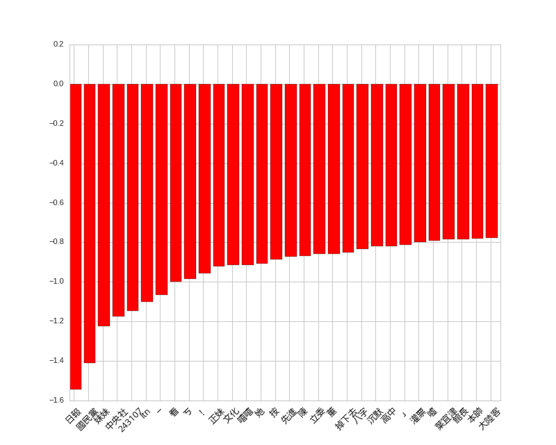
Firstly, let’s see the negative words in posts. Not sure why, but when the posts mention 妹妹, they are more likely to attract negative responses.

# top features for posts
display_top_features(svc.coef_[0], dvec.get_feature_names(), 30)

Negative Words in Posts

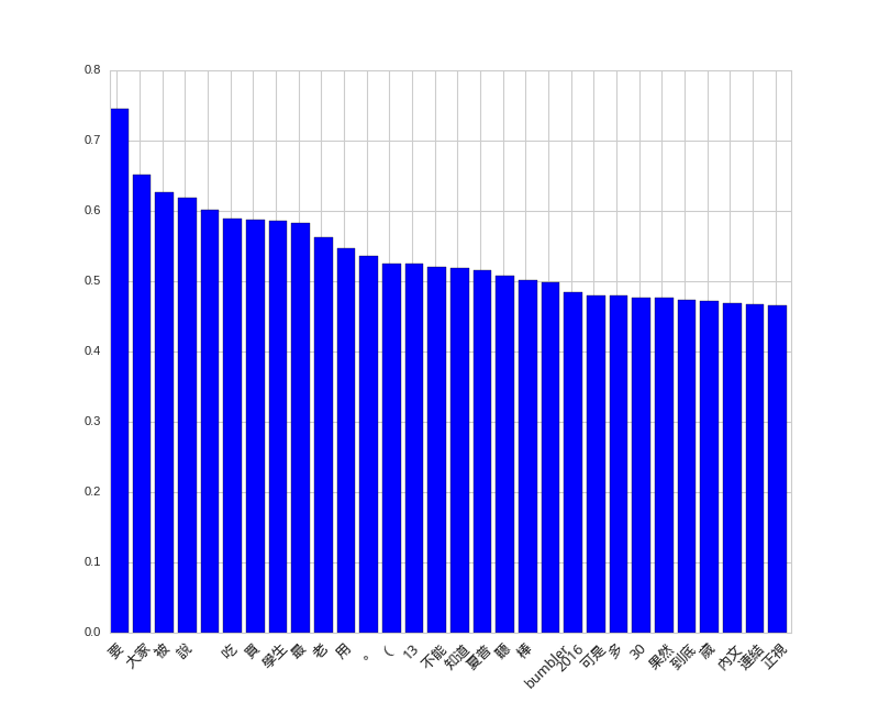
Unfortunately, no interesting patterns are observed for positive words in posts.

# top positive features for posts
display_top_features(svc.coef_[0], dvec.get_feature_names(), 30, select=lambda x: x)

Positive Words in Posts

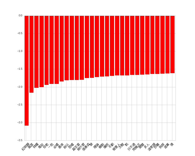
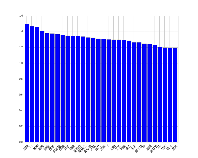
The positive and negative words in comments are very interesting, the strongest features are 紅明顯 and 給推.

# top features for comments
display_top_features(c_svc.coef_[0], c_dvec.get_feature_names(), 30)
# top positive features for comments
display_top_features(c_svc.coef_[0], c_dvec.get_feature_names(), 30, select=lambda x: x)

Negative Words in Comments

Positive Words in Comments

Conclusions

Although many years have passed, Python 3 support still has not reach desired states, but it’s already getting better. Hopefully more people will start programming in Python 3.

After I’ve finished the analysis, I feel that PTT is really a great place to learn about the current topics people are interested about in Taiwan. Not sure whether there will be other applications.

The code used in this experiment is on GitHub for reference: https://github.com/shaform/experiments/tree/master/scrapy.

Links

If you like this article, you might also be interested in 〈Scrapy Cloud + Scrapy 網路爬蟲〉.